Predicting Patterns of Play
Introduction
Football is a game where anything can happen…or is it? A free-flowing game where 22 players change positions constantly with respect to a ball may sound and look like chaos. Statistically, the sheer amount of different combinations of players, locations and actions is overwhelming. Most series of events are never truly repeated. In the rare instances where an event sequence is exactly replicated during a game, usually too much has happened in between that one can easily not acknowledge it. This can make a game of football appear chaotic and often, to the untrained eye, games look like a collection of random events for 90 minutes. However, football teams spend countless hours in preparation. Tactics are being discussed and adopted. Training sessions are commenced where players are drilled into recognising certain game situations and applying manager-approved protocols into solving them. In theory, a team should have protocols for dealing with any state the game is in, applying principles which are coached by the coaching staff. In reality, one can not prepare for all possible game state, player and location combinations as they are simply too many in a game of football. The discrepancies between the two are where the randomness in a football game commences. However, if the randomness is ignored, the pre-prepared protocols that the team has been drilled to execute are left and finding these will be the aim of this article.
The Markov Process
The team that will be analysed is Chelsea WFC and its 20/21 season. The question that the article will attempt to answer is ‘What are the protocols of Chelsea WFC’. The analysis will focus only on what the processes are and not why or when they are applied. In the process of answering that question, a Markov chain will be created containing all events and their locations.
A Markov process is a process where predictions can be made regarding future outcomes based on the current state of play. In a given sequence of events, it iterates through each event where for each iteration it pairs the event with its descendant, labelling the first ‘current state’ and the latter ‘subsequent state’. Each state has a list of all the different states (including itself) it can lead to and their frequency, forming a probability of going from it to another one. In the end, random sequences will be generated with an algorithm using those probabilities to form the most probable series of events given a certain event-location is the start.

Markov chains are characterized as ‘memoryless’ meaning that they generate the subsequent event only based on the current one and not on the ones before that. In the context of football, this approach will not provide the full context as it matters whether a player for example receives the ball from a short pass on the ground or from a 40m long ball. More accurate models exists that take those considerations into account and they will be explored in future articles. However, for the purpose of the analysis, the Markov model will be explored in its memoryless form.
Methodology
The dataset that will be used is the WSL 2020/2021 season data provided by StatsBomb free data repository. All games that Chelsea WFC have played have been filtered in order to produce a dataset of events which occurred only during their games. Several assumptions have been made to aid the analysis, namely:
1. The pitch has been split into 30 zones
Analysing the coordinates of each event independently would not yield any insights due to the variable nature of event coordinates. Hence, the pitch has been split into zone containers each representing a certain range between X and Y coordinates. Figure 1 outlines the zones in which the pitch was split. The zones split the pitch into 6 laterally in order to break down the opposition half into 3rds and into 5 longitudinally in order to include the half-spaces which have become popular in modern football.
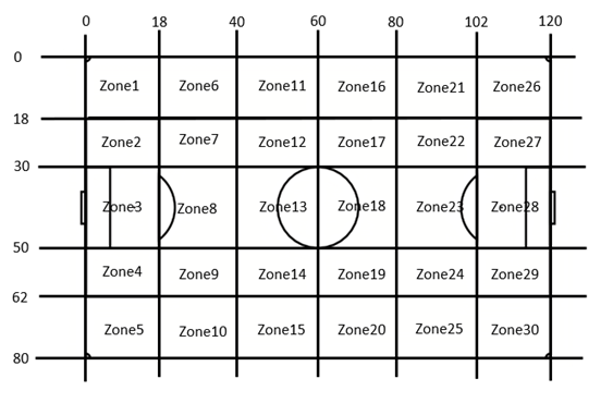
Events have then been added to their respective containers. This forms a link between the event and the zone it happened which will be represented in the following format:
{Event Type} — {Event Zone}
An example possession would look like the following:
(Pass-Zone6) -> (Interception-Zone9) -> (Carry-Zone9) -> (Pass-Zone9) -> (Carry-Zone3)
1. Dribble and Ball Receipt events have been filtered out from the dataset
Both have been deemed to not add extra value over using just the Pass event in the context of the analysis. Every Pass has a Ball Receipt linked to it which is very rarely positioned in a different zone to the next event, making it redundant. Just like passes are coupled with ball receipts, in the dataset used, every time a ‘Dribble’ event occurs it is coupled with a ‘Carry’ event. Upon inspection, it was determined that ‘Carry’ events provide more information in the context of the analysis and were kept over ‘Dribble’ events
2. Possessions against Chelsea have been filtered out
Since the purpose of this analysis is to concentrate on predicting what Chelsea WFC do when they are in possession, all possessions from other teams have been excluded from the dataset to avoid misleading results.
Once the dataset has been cleaned, all the event-zone combinations have been added to a list. This list is then iterated through to create a Markov model containing the probabilities of advancing onto any other event-zone combination given the current state. For the purpose of this exercise, this will be sufficient in order to generate stories.
To generate a random possession, a starting state will need to be passed onto the algorithm as well as the length of the sequence we want to generate. The algorithm will then use the probabilities that have been generated from the Markov model to create a passing sequence to the desired length. In theory, any event-zone combination can be passed as a starting state, but for the purpose of this analysis, only four states will be looked into. Similarly, a possession of any length can be generated and for this analysis, the assumed length of a possession will be five events. Lastly, nine hypothetical possessions will be generated for each state.
The only step left is to define the states of interest. For this purpose, a heat map, containing all the events during the 20/21 season will be used to determine the most used zones from the team.
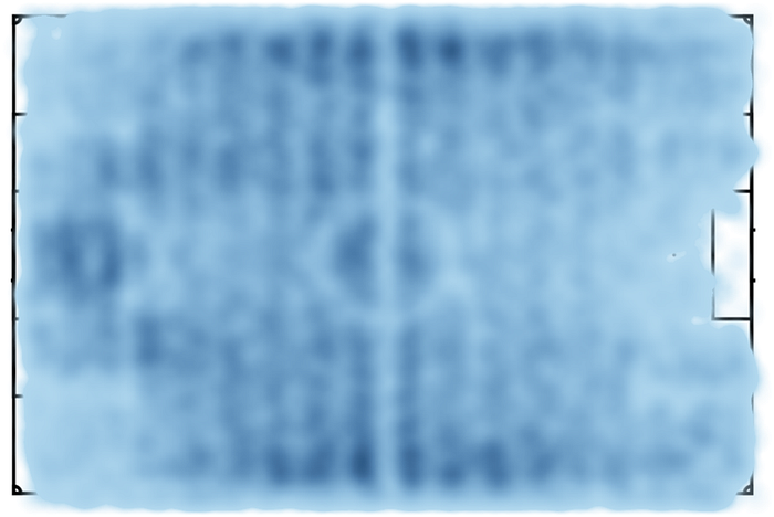
Figure 2 outlines the commonly used areas by the team while in possession. It can be seen that Chelsea has made use of Zones 11,16 on the left-hand side and Zones 15,20 on the right-hand side. Only zones 16 and 20 will be used as states as they are closer to the opponent’s goal. On top of those 2 zones, passes from Zone 3 will be included in order to represent a probable sequence of events following a goal kick from Chelsea, as well as Zone 21, considered to be one of the zones most frequently leading to a shot as per the previous article.
Results
Pass-Zone 3
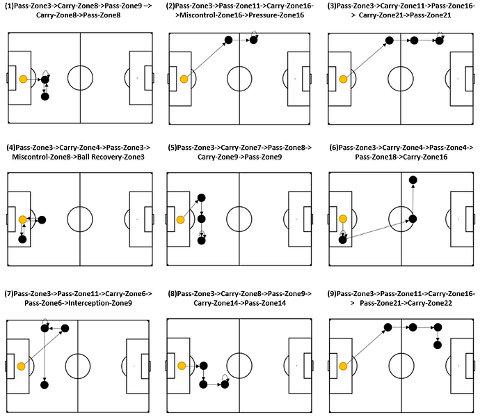
Looking at the nine hypothetical cases that have been generated from the algorithm for ‘Pass-Zone3’ it can be seen that there is an equal spread between resolving to play out from the back and making the decision to play over the first line of the opposition directly to the middle 3rd. An interesting trend can be observed when the team do decide to play over the first line of defence, they mainly resolve to playing in Zone 11 which is on the left-hand side of the pitch. Looking further into the sequence, once the ball reaches Zone 11 it is being progressed forward through the wide areas into Zones 16 and 21 with only one occasion where it is being passed back and recycled(7). When a decision is made to play out from the back, rather unsurprisingly the following four plays do not progress the ball further onto the pitch but is played between players in the zones in front of the goal, possibly to force a reaction from the opposition.
Pass-Zone16
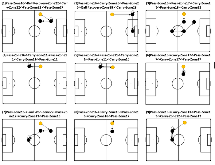
The generated sequences starting with Pass-Zone16 show a preference for slow build-up instead of a direct approach. Upon inspection, only one sequence (2) presents an attack which ends up in Zone 28. Instead, the algorithm insists that it is more likely for the team to make short passes in the attempt to consolidate possession or to move the ball to the other side of the pitch. There has also been a lack of long ball switches from the left-hand side to the right-hand side which serves as a further indication of the team’s preference to play short passes when in that area.
Pass-Zone20
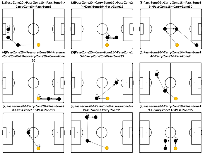
Similar to the previous case, Pass-Zone20 offers little difference in principle to what was observed when the team was in a similar position but on the other side of the pitch. The most probable sequence in this area consists of short passes which aim to consolidate possession or to switch the area of play to the other side of the pitch. Two outliers are presented in (3) and (5) which show attempts for a more direct play.
Pass-Zone21
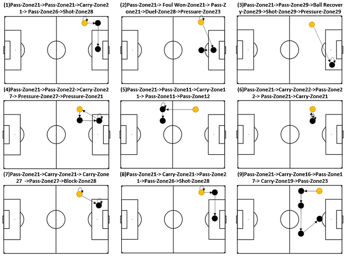
Looking at Pass-Zone21 becomes more interesting as the area is positioned in the attacking 3rd of the pitch and one would expect to see more assertive plays to attack the opposition goal. And indeed a shot has been included in the sequence in three (1),(3), and (8) of the nine generated samples which can serve as an indication of the team’s potency to create a shooting chance from that area. In those cases, the shot has been preceded by either a cross (1),(8) or a switch into the opposite half-space, something that could be worth analysing in depth. It can also be observed the high presence of Pressure events which can serve as an initial indication of counter-pressing tactical instructions in the final 3rd.
Conclusion
In competitive sports, every piece of information can be used to gain an edge over the opponent. As eluded to in the previous article, having a better initial understanding of the thought process of an opponent can vastly decrease the amount of time spent on preparation by narrowing down the topics for detailed analysis. Alternatively looking at one’s own team such analysis can serve as an additional check of the effectiveness of preparation or the quality of execution.
In this article, a season-long dataset of events for Chelsea WFC has been analysed and a Markov chain has been constructed to calculate the probabilities of transitioning from one state to another. This has then been used to simulate possessions with a pre-determined starting point. For the purpose of the analysis 4 starting points have been analysed namely: a goal kick Pass-Zone3 passes starting in the most active areas for the team Pass-Zone16 and Pass-Zone20 and passes from an area determined to be potent for creating shots Pass-Zone21. By running only nine simulations, some potentially interesting insights can be observed like the team preferring to pass to the left-hand side of the pitch if it makes a decision to skip the first line of defence or that when in Zone20 or Zone16 the team would rather consolidate possession than look for a direct approach. Pass-Zone21 had 30% of its simulations ending with a shot which confirms its potency to create shots, it also visually recreated the way that is most likely for the team to create a shooting chance — with crosses.
Markov chains are stochastic in nature and only nine simulations are not a big enough sample size to reach any conclusions. Having a higher number of simulations would generate a set of sequences which would together contain a more accurate representation of what a given team is capable of. Those can then be labelled and fed into the coaching staff providing the insights that could allow for a better understanding of the analysed team.
In this case, five events in total have provided satisfactory results but they can be changed to reflect the needs of the user.
The accuracy of the probabilities can be further increased by taking into account the action that led to the current state, however for that to be feasible, a bigger dataset is required.
Time is a precious entity and that is even more true when in a competitive environment where efficient use of time can lead to better results. Luckily for us, computers can do the hard work of analysing tens of thousands of data points and presenting it into a digestible format. Having a tool that can present the N most probable sequences starting from a pre-defined condition can be expanded to include set-piece patterns. It can enable teams to focus on the details quicker, something which in the long run can make the difference.
Comments
Post a Comment