How to know your opponent better
Introduction
Football is a subjective sport. Everyone can have an opinion on the way a team plays or the style of a certain player. And whilst it is entertaining for fans to speculate on certain topics, it is crucial for people working within the game to have an exact classification of what they are working with and this is where objective decision-making has its merit.
Objective decision-making is already embedded into football physical performance analysis. Teams have used data to decide on players‘ physical capabilities before making an informed decision on whether a certain player would be a good fit. Whilst physical capabilities are essential to a player’s or a team’s performance, there are technical, tactical, and social considerations that one has to take into account before making a conclusion. A player may have exceptional performance indicators in a certain environment but underperform in another. Player roles are well documented and there are numerous theories on play styles and the type of players that are required for them to function. However, not having an objective measure means relying on subjectivity and its inherited bias for the majority of what makes a player or a team. And that is not a great place to be.
This analysis will attempt to use LSTM models to classify the playing styles of teams based on possession sequences. Three main categories will be defined which represent the main styles of play that a team can produce namely Slow build-up, Direct play and Control based play. Two more categories are added in Set-pieces and Uncategorized to allow for isolated events and less organized sequences to be classified.
LSTM Neural Networks
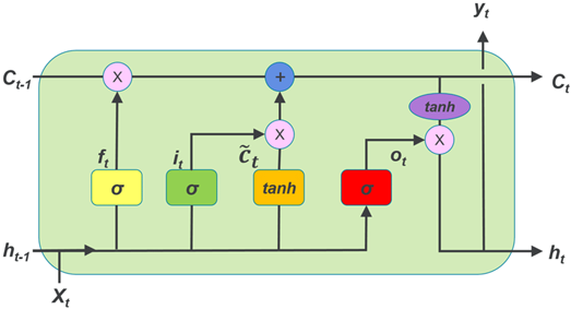
Long short-term memory is a type of recurrent neural network that can process not only single data points but also entire sequences of data. The name is derived from having the ability to store and take into consideration information not only from short-term memory but also retained information from previous states called ‘long-term memory‘.
LSTM models have 3 gates and 1 state:
The cell state is used to store the ‘long-term memory’. It starts from the beginning of a cycle, gets updated if necessary, and then is used in conjunction with the input to produce an output.
The forget gate is used to update the cell state in the beginning. It takes into consideration the input and the ‘short-term memory’ from the previous event and updates the cell state accordingly.
The input gate is used to add information from the new event to the previous knowledge in the cell state.
The output gate takes into consideration information fed from the cell state combined with the previous output data to return a new output.
Methodology
1. Labelling sequences
The labels are one of the most important decisions that need to be made in a classification exercise. In football, teams can have
Slow build-up — A sequence containing more than 5 short-medium length passes which aim to advance the ball into dangerous areas.
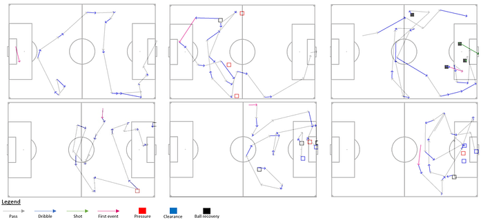
Set-Piece — Free-kicks, Corners, Throw-ins
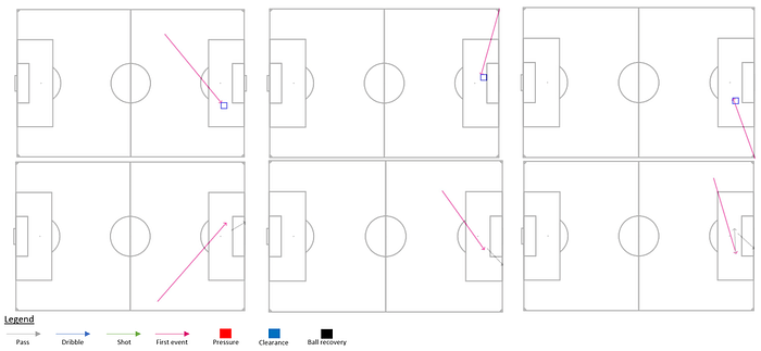
Direct — A sequence that contains mainly forward passes which aim to progress the ball into dangerous areas as quickly as possible.
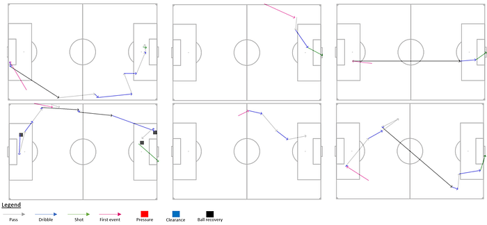
Control — A sequence containing many forward and backward passes which aim to keep the current state of the game.
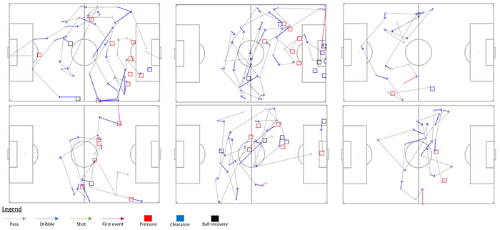
Uncategorized — Sequences that do not fall under any of the other four categories.
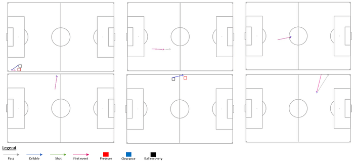
2119 sequences in total from season 20–21 season have been labelled
1. Prune event information
Each event in the database contains 173 pieces of information which would be computationally demanding if used without any adjustments. For this reason, a focus has been given to information that is critical to identifying the playstyle, namely:
Type of event, play pattern, player position, pressure, location of events and various crucial details about specific event types like pass length, pass height etc. After pruning was performed, the information for each event was reduced to 33 pieces of information.
2. One-hot encoding all categorical information
As big part of the data comes in categorical textual format, encoding needs to be performed. Most of the textual data is in a nominal form and is, therefore, one-hot encoded. One-hot encoding avoids the hierarchical assumptions of other type of encodings which are mainly targeting ordinal data. There were also Boolean values which would be mapped as 1 if true and 0 if false.
3. A threshold of 60 events per sequence has been established
Out of all 2119 sequences, there were only 8 sequences above 60 with the highest being 79 events. In order to increase efficiency, those 8 sequences have been excluded from the analysis.
4. Balancing labels
The initial labelling of playing style indicates that there is an imbalance in the label occurrence as outlined in figure 3.
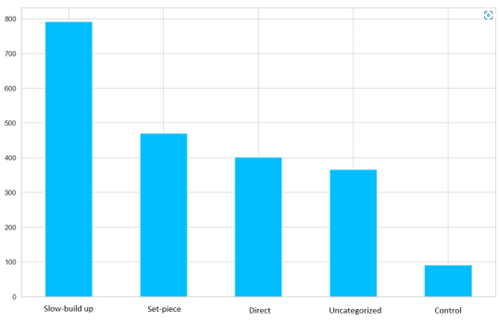
Slow build-up is almost 8 times more frequent than Control. An oversampling has been applied by resizing each label to achieve a more balanced distribution.
After being balanced, the dataset was split into training and testing with an 80/20 split and a dictionary was created from the tensors of the sequence and its respective label. Finally, an LSTM model has been applied using PyTorch and PyTorch with cross-entropy has been used as the loss function.
Results
Results from the LSTM model are presented in Figures 2 and 3. A high validation accuracy has been achieved with 91%. However, it can be seen that validation loss is higher than training loss, with the minimum loss achieved is 39%. It remains stable at around 40–45% which is a positive sign that the model does not overfit. The relationship between accuracy and loss indicates that although the absolute prediction is accurate most of the time, the model is not confident in it. That kind of behaviour is to be expected due to the high variability of the data inputs and the lack of a strong definition of each label.
Different scenarios have been run as shown in figures 2 and 3 trying to improve the validation loss. However, it can be seen that results remain pretty stable across all four different scenarios.
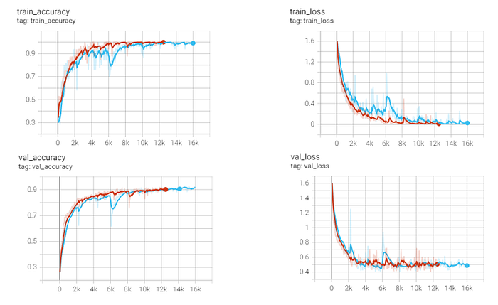
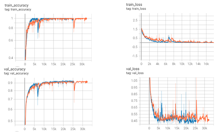
The achieved validation loss will be deemed satisfactory due to the nature of the analysis. As discussed above football playing patterns do not have a specific definition. They are open to interpretation and are heavily dependent on context. Even though an attempt has been made to define a set of rules to aid labelling, the highly varying nature of the sequences decreases the confidence in the predictions. Moreover, in this analysis, only the critical information to identify the event location and type has been included. Working with a bigger sample size would allow for more context-defining variables to be included which should, in theory, help the model in its predictive confidence. Results shown from the confusion matrix in Figure 4 show that slow build-up is the one with the lowest accuracy and is mostly mistaken for direct or control play styles. This is to be expected due to the fact that both playing styles can be quite similar to each other when taking into account only event coordinates and event count. However, even without including context, the model was able to predict correctly almost 80% of the time. Uncategorized data was mostly mistaken for direct plays and set-pieces. This could be because some of the labelled direct plays and set-pieces contain only one event which is most of what the uncategorized labels are made of. It can be observed that direct plays are not mistaken for control plays, mainly due to the fact that by definition, one play style should presumably contain much shorter sequences than the other, something which the model has recognized. Lastly, it can be seen that control plays have been predicted 100% of the time, which could be largely due to oversampling that was done earlier.
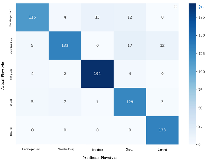
The predictive power of the model can be enhanced by including information on the context of a particular sequence. Information like the types of passes (differentiating between risky and safe) or pressure applied could significantly improve the model. Furthermore, more specific definitions for labelling could also increase the confidence in which the model predicts.
Conclusion
The higher the level that football is played, the smaller the differentiations that separate the winners from the losers. The more difficult it becomes for the naked eye to spot and pinpoint an objective reason for a certain outcome. Moreover, no human can catch all details in a game and even experienced professionals would require highly concentrated efforts before labelling certain playing sequences and reaching the stage where they ask the right questions. Having a tool which significantly shortens the amount of time needed to ask the right questions would allow analysts to spend more time finding the answers to those questions.
An LSTM model was used to classify possession sequences into playing styles. The achieved accuracy was 91% on the best iteration and the loss was 40% which, considering the complex nature of the sequences, was deemed to be satisfactory.
Such models outline initial steps towards being able to objectively classify complex datasets such as the ones of a free-flowing game of football. The same approach can be used to classify specific events which teams would like to bring attention to during opposition or team analysis. It could also be used towards understanding the habits of players and putting them into a category which can then be used to assess if one is a good fit for a certain system.
Attention is brought to many events or sequences that share similar contexts and are classified as being the same in an efficient manner, without needing to spend a vast amount of time. The saved time can then be utilized to break them down to the finest details and then find patterns to be able to come close to the way people involved in the decisions think and more importantly maybe uncover more pieces of the puzzle towards a certain outcome. Something which in the long run can make a difference.
Comments
Post a Comment